1Introduction
Distributed rate limiting is usually solved with a centralized counter. A node receives a request, makes a synchronous call to Redis or a similar datastore, and gets back an exact global count. The approach is correct, well understood, and widely deployed. It is also a bottleneck: every request pays the round trip, every counter update goes through the same hot key, and the central store is a single point of failure that the CAP theorem forces you to choose between availability and consistency on.
This writeup explores what happens when you remove the central authority entirely and replace it with gossip. Each node keeps its own G-Counter CRDT for each key, increments it locally on every admitted request, and periodically sends its counter deltas to a handful of random peers. Counters converge eventually; no synchronous coordination is required on the request path. The tradeoff is that during the convergence window, nodes make admission decisions against a stale global count, and some requests slip through. The central question of this writeup is how to bound that error, and then how to drive it down below the level where anyone would notice.
The analysis here is framed around rate limiting, but the underlying dynamics are general. Anything built on epidemic gossip faces the same convergence-versus-bandwidth tradeoff, and the machinery developed in the next few sections (the over-admission bound, the two-stage adaptive interval, the adaptive fan-out, and the convergence analysis) applies to any system where stale state has a measurable cost.
1.1 What This Tab Covers
Section 2 defines over-admission, derives the worst-case bound during a coordinated burst, and shows why the error scales linearly with request rate. Section 3 builds up the adaptive gossip protocol one component at a time: starting from a static interval, introducing pressure-tiered gossip, velocity-continuous gossip, their multiplicative combination, and finally adaptive fan-out. Section 4 ties the pieces together with a probabilistic convergence analysis that predicts, for any given system state, how long a delta takes to reach the rest of the cluster. Section 5 validates the theory against 1,680 benchmark runs on a 25-node Docker cluster and shows that the adaptive protocol strictly dominates fixed-interval gossip on the accuracy-bandwidth Pareto frontier.
For implementation details (the Rust binary, the CRDT store, the gossip transport, SWIM-based membership, and the performance numbers), see the Architecture tab. The analysis and the implementation were developed in tandem, but the analysis stands on its own and does not require any of the architecture content to follow.
1.2 Contributions
The core contributions are two analytical results and one empirical one. First, an efficiency metric showing that over-admission per gossip message is proportional to (interval over fan-out), which collapses the two-dimensional configuration space onto a single axis. Second, a two-stage multiplicative formula that lets pressure and velocity jointly compress the gossip interval, combined with a shaped adaptive fan-out that raises the log base of the convergence bound exactly when headroom is smallest. Third, a 1,680-run benchmark sweep (21 configurations, 4 load profiles, 2 traffic distributions, 10 iterations) on a 25-node cluster showing that the adaptive protocol Pareto-dominates fixed-interval gossip across every burst profile tested. The convergence bound itself is not new (it follows from the standard epidemic infection model), but plugging the adaptive controls into it and showing that the resulting convergence time tracks the application's actual risk profile is the contribution that ties the whole thing together.
2Over-Admission Bounds
The entire purpose of using gossip this way is trading perfect consistency for speed. That's great and all but it sounds a bit scary until we answer the question: how many extra requests actually slip through during the convergence window?
2.1 Defining Over-Admission
Over-admission is the number of requests admitted cluster wide beyond the configured limit before counters converge. It happens because during the gossip convergence window, each node only sees its own local count plus whatever it's received from peers so far. If requests hit multiple nodes simultaneously, each node underestimates the true global total.
The worst case is simple: all N nodes receive requests for the same key at the same time, and none of them have synced yet. Each node thinks the global count is just its own local count. The over-admission window lasts until gossip propagates the counts to every node, which we know takes approximately .
The maximum over-admission during a coordinated burst across all nodes:
where is the aggregate request rate across the cluster, is the gossip convergence time, and is the number of nodes.
The intuition: during the convergence window, each node is blind to of the total traffic. The total number of requests that arrive during that blind window is , and the fraction that's invisible to any given node is .
Say a certain key has a rate limit of 1000 requests per minute, distributed evenly across 5 nodes. Each node receives 200 requests per minute, or about 3.33 requests per second. Our convergence time with N=5, K=3, and T=100ms is approximately 200ms. During that 200ms window, each node admits requests without full visibility of what the other 4 nodes are doing. The math:
- Requests arriving per node during convergence: 3.33 req/s * 0.2s ~ 0.67 requests
- Each node is blind to 4 other nodes' traffic
- Total over-admission: 0.67 * 4 ~ 2.67 requests, so roughly 3 extra requests
For a limit of 1000 requests per minute, 3 extra requests is a 0.3% overshoot.
2.2 Stress Testing at Scale
Now let's stress this at scale. Same 5 nodes, same K=3, same 200ms convergence window, but now the rate limit is 1000 requests per second. This is a realistic throughput for a high-traffic API gateway or a CDN edge node handling authentication tokens.
With traffic distributed evenly, each node handles 200 requests per second. During the 200ms convergence window, each node admits requests with no visibility into the other four:
- Requests arriving per node during convergence: 200 req/s * 0.2s = 40 requests per node
- Each node is blind to 4 other nodes' traffic
- Total over-admission: 40 * 4 = 160 extra requests
That's a 16% overshoot. 1160 requests admitted against a limit of 1000. And this is the average case with perfectly uniform distribution. If traffic is skewed (which it always is in practice, think geographic hotspots or retry storms), the problem compounds. Two nodes receiving 80% of the traffic will each locally see 400 req/s, blow past the limit independently, and not learn about each other until 200ms later.
The core issue is that the over-admission bound scales with the request rate. At 1000/min, 200ms of blindness costs you 3 requests. At 1000/sec, that same 200ms costs you 160. The convergence window didn't change. The traffic filling it did. This is where a static gossip interval fundamentally breaks down.
2.3 The Over-Admission Ratio
To generalize beyond a single example, define the over-admission ratio as the fraction of excess requests relative to the configured limit over a full window:
where is the configured rate limit. In terms of system parameters:
This ratio stays bounded and predictable as a function of your gossip parameters. If you need tighter bounds, you have three knobs you can fiddle with: decrease the gossip interval T (converge faster), increase the fanout K (converge faster), or accept that the bound is already negligible for your use case.
What's really important is that scales with , which scales with . So as you add nodes, the over-admission window grows logarithmically, not linearly.
2.4 When Does This Actually Matter?
For most rate limiting use cases (API throttling, DDoS protection, etc), a sub-1% overshoot is completely acceptable. The rate limit exists to prevent abuse, not to enforce a mathematically perfect boundary. If your limit is 1000/min and you occasionally admit 1003, nobody notices.
Where it gets interesting is at the extremes. If your rate limits are very tight (say, 10 requests per minute), the same 3-request overshoot is now a 30% error. And if your cluster is large (50+ nodes) with high aggregate traffic rates, the convergence window admits proportionally more excess requests.
For those cases, there are two mitigation strategies. The first is the adaptive gossip approach I'll cover later: gossip faster when counters are close to their limits, which shrinks when it matters most. The second is a hybrid approach: process 99% of requests via the fast, lock-free CRDT path, but inject a synchronous coordination barrier when a key's count crosses a safety threshold (say, 90% of the limit). This gives you the latency benefits of eventual consistency for the common case while enforcing strict accuracy at the boundary.
The absolute counting error at any node is bounded by:
where is the request rate at node and is the expected propagation delay from node to the observing node. Under uniform load and symmetric gossip:
This bound comes from the concept of Probabilistically Bounded Staleness (PBS), formalized by Bailis et al. Rather than treating consistency as a binary (strong vs. eventual), PBS models it as a continuous gradient where staleness is a function of network latency and gossip parameters. In our system, the "staleness" is exactly the over-admission count.
3Adaptive Gossip
Convergence time is how long it takes for a piece of information to reach every other node in the cluster via gossip. If node 1 increments its counter, convergence time is the duration until node 25 has seen that increment. For example, with 25 nodes, a random fanout of 3, and a gossip interval of 200ms, convergence takes around 2-3 gossip rounds, so ~400-600ms. The cluster is essentially "blind" during this convergence window. Think of different gossip intervals, and a ton more nodes. If you have say 150 nodes in edge environments on the cloud with a gossip interval of 1 second, and average latency of around 100ms to hit each node, you're looking at several seconds of blindness, which is unacceptable in high traffic systems with high request rates. This is where the question comes up: what the heck can we do about this? Gossip seems like a really interesting protocol for distributed systems, but can we really handle this much error? One idea that pops up is what if we can adapt the gossip interval given certain parameters?
3.1 Why Static Gossip Wastes Bandwidth
In this system, a static gossip interval has some pretty bad drawbacks. If every key gets the same gossip frequency, a key at 5% utilization getting gossiped every 200ms is just wasted since peers already know its state, and even if they didn't, who cares - it's not near the limit. A key at 95% utilization needs more frequent gossip than 200ms because every request that slips through during the blind window is a real over-admission. The only knob available is the global interval, and turning it up helps accuracy but scales bandwidth with 1/interval across all keys, not just the ones that matter.
To see this concretely, I swept the gossip interval from 100ms to 6000ms on the 25-node cluster under steady 8x load and plotted the results:
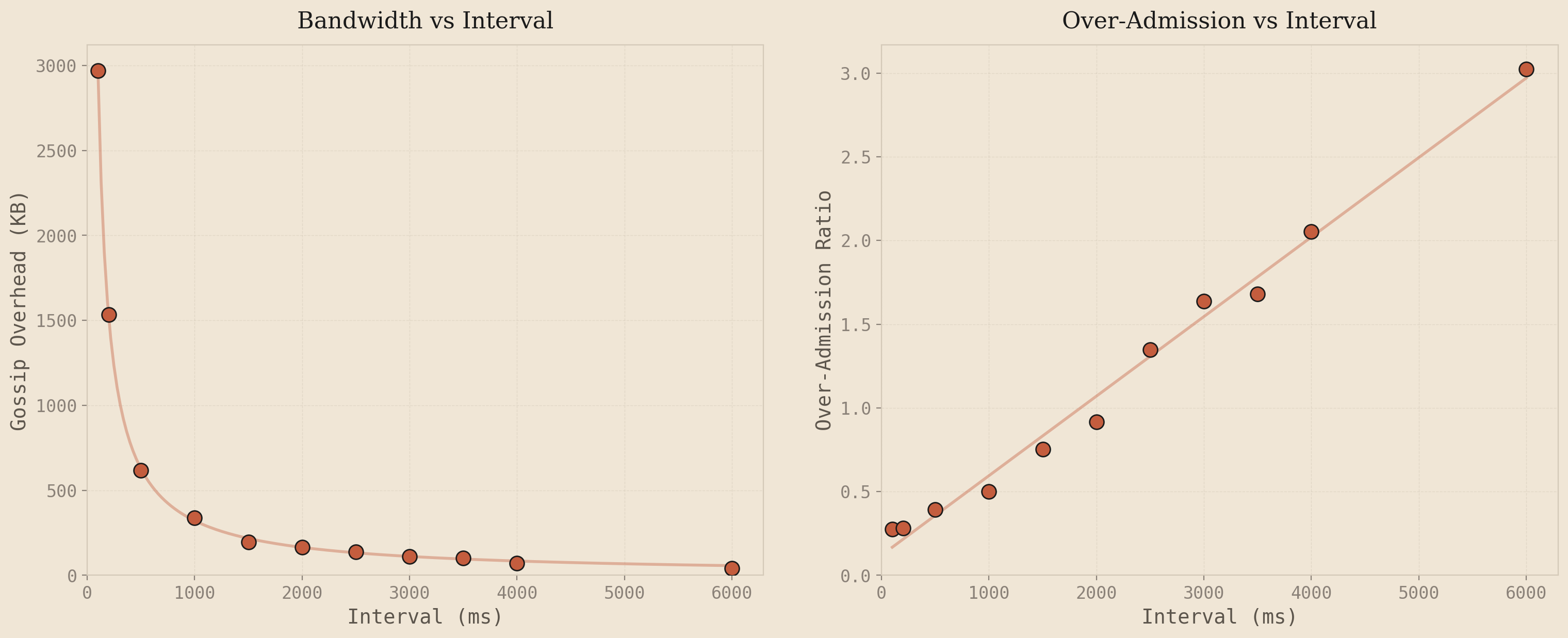
The left plot shows gossip bandwidth dropping as a negative exponential as the interval increases - gossip every 500ms fires 40 rounds in a 20-second test, gossip every 4000ms fires 5. Fewer rounds, fewer bytes. The right plot shows over-admission growing linearly with the interval. This falls directly out of the over-admission bound from Section 2: . Convergence time is proportional to the gossip interval, and everything else is constant, so OA scales linearly with the interval.
These two curves are the entire problem. You want to be in the bottom-left of both graphs simultaneously - low over-admission and low bandwidth. But the only knob is the interval, and moving it helps one axis while hurting the other. Bandwidth drops as , OA grows as . There's no interval value that gives you both. That's the no free lunch problem with static gossip - and it's why the interval needs to respond to traffic conditions instead of being a fixed constant.
3.2 Pressure-Tiered Gossip and Why It Fails
The natural first idea is to gossip hot keys more often than cold ones. Define pressure as a per-key metric: . A key at 270/300 has pressure 0.9. A key at 30/300 has pressure 0.1. Assign keys to tiers based on pressure, and give each tier its own gossip interval:
where is the base interval, is the pressure at tier , and controls the curvature
The implementation is straightforward: the sender loop ticks at the fastest tier's interval. On each tick, it checks which tiers are due and only sends keys from those tiers. High-pressure keys piggyback on every round via an inclusive rule - if any tier is due, keys at tier get included. The intuition is that keys close to the limit need the cluster to converge on their count as quickly as possible, while keys far from the limit can afford to wait.
I swept tier counts from 1 (fixed-rate baseline) through 10 across five gossip intervals on the 25-node cluster under steady 8x load. The results:
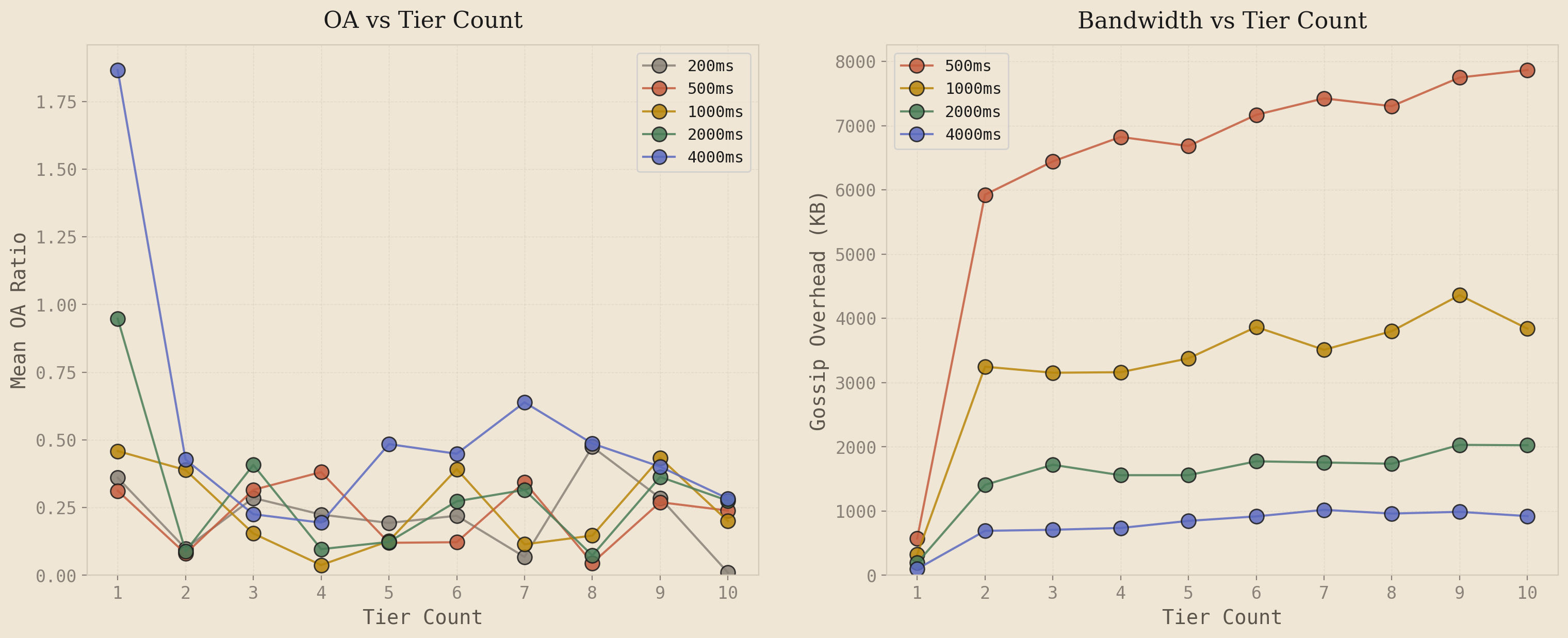
The left plot tells the story. Going from 1 tier to 2 tiers drops OA noticeably - the fast lane catches keys approaching the limit and gossips them more frequently. But beyond 2 tiers, the lines go flat and noisy. 3-tier, 5-tier, 8-tier, 10-tier all bounce around the same OA range with no consistent improvement. Adding more tiers does not help because under uniform load distribution, every node sees roughly the same pressure for a given key - about for steady 8x. Intermediate tiers never activate meaningfully because all nodes fall into the same tier. The system degenerates into a 2-tier binary: fast lane or slow lane.
The right plot shows what those extra tiers cost. Bandwidth jumps 8-10x the moment you go from 1 tier to 2 tiers, then plateaus. The fast tier dominates the gossip volume regardless of how many slower tiers you add below it. You are paying for the infrastructure overhead of tier management with no accuracy benefit.
But the deeper problem is not the tier count - it is the signal itself. Pressure measures how full the bucket is, which is a staticproperty. What matters for gossip scheduling is how much a node's local state has diverged from what its peers know, which is a dynamic property. Consider two scenarios:
A key sitting at 90% utilization with no new requests for 10 seconds. Every peer already knows the count from previous gossip rounds. Gossiping this key again sends the exact same state the peers already have. It is a wasted message. But pressure-tiered gossip assigns it to the fast tier because 90% is "high pressure."
Now consider a key at 20% utilization that just received a burst of 50 requests in the last 100ms. No peer knows about these 50 requests yet. The local state has diverged significantly from peers' estimates. This key urgently needs to be gossiped, but pressure-tiered gossip assigns it to the slow tier because 20% is "low pressure."
Pressure tells you where you are. What you need is how fast you are moving - because the rate of change is what determines how quickly your local state diverges from your peers' estimates. A node sitting at 90% with zero velocity has zero divergence. A node at 20% with high velocity has maximum divergence. This distinction - between static state and dynamic divergence - is why we need a different signal entirely.
3.3 Velocity-Continuous Gossip
The alternative to pressure is velocity: the exponential moving average of the local request arrival rate for a key. Velocity measures how fast the local counter is changing right now. If requests are arriving at rate on this node, then the local counter is incrementing at rate . Peers don't know about these increments until the next gossip round. So the divergence between local state and peers' estimates grows at approximately per unit time. High velocity means high divergence rate means urgent need to gossip.
Instead of discrete tiers, the gossip interval becomes a continuous function of velocity:
where is the base interval, is a sensitivity parameter, and is the velocity EMA. Floor: .
The mechanics are straightforward. When (no traffic), and gossip fires at the base rate, same as fixed. When velocity is moderate, shrinks proportionally - more traffic means faster gossip. When velocity is very high, approaches the floor at 50ms, the maximum gossip rate. And when traffic stops, decays via the EMA and relaxes back to .
No tiers. No tier boundaries. No promotion latency. The interval is a continuous function of the local arrival rate. The sender loop reads the max velocity from the CRDT store, computes , sleeps for that duration, and ships all dirty keys. The intelligence is entirely in when rounds fire, not what they contain.
The velocity itself is tracked as an exponential moving average, updated on every increment:
1// Updated on every increment2let dt_ms = now.duration_since(vel.last_update).as_millis() as f64;3if dt_ms > 0.0 {4 let instant_rate = hits as f64 / dt_ms;5 vel.ema = velocity_alpha * instant_rate6 + (1.0 - velocity_alpha) * vel.ema;7 vel.last_update = now;8}
One subtlety worth noting: the EMA only updates when requests arrive. If traffic stops completely, the EMA would hold its last value forever, keeping the gossip interval compressed indefinitely. To handle this, the velocity read path applies passive decay based on elapsed time since the last update. When the sender loop calls max_local_velocity(), the returned value is where is the time since the last increment. This ensures the interval relaxes back to baseline even during complete silence.
The parameter controls how aggressively the interval responds to velocity. Higher values mean the interval compresses faster for the same arrival rate. In practice, in the range of 1000-10000 works well depending on cluster size and target limit. The effective sensitivity scales with the number of nodes and the aggregate request rate.
To visualize how this works in practice, I ran a 5-node cluster through a three phase test: 5 seconds of silence, 5 seconds of burst traffic at 500 requests per second, then 5 seconds of silence again. The plot shows the velocity EMA and the resulting gossip interval across the cluster:
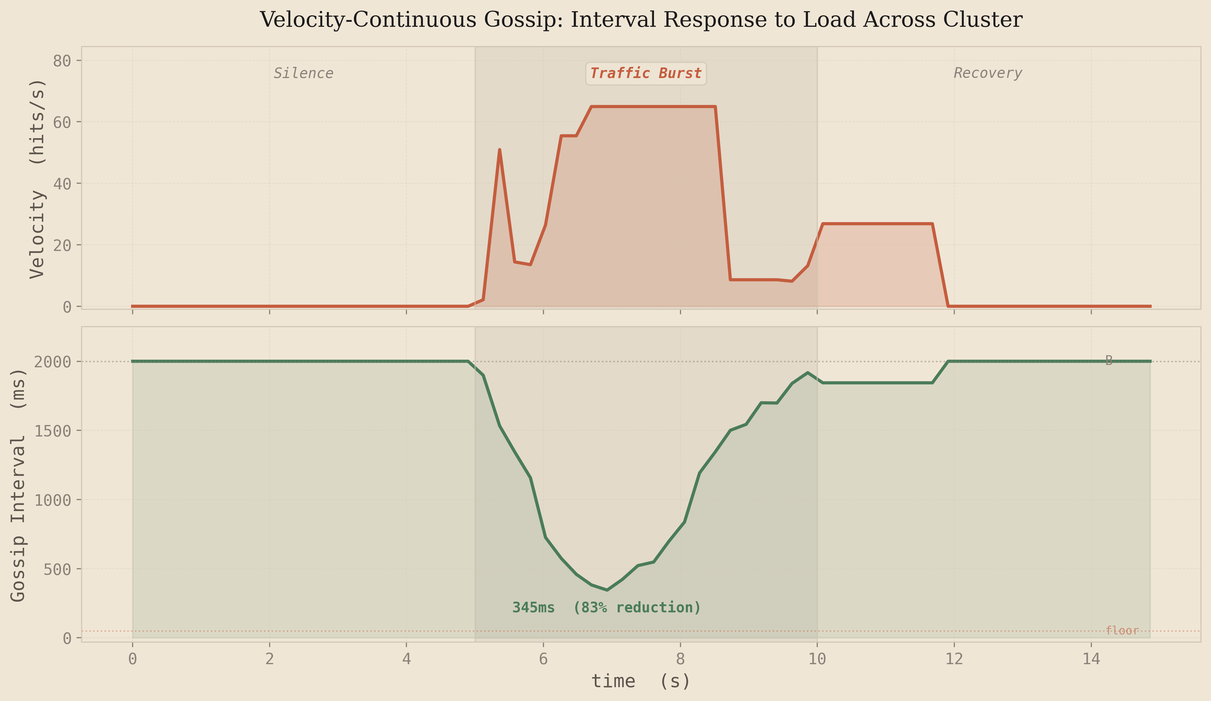
The behavior is exactly what you'd want. During the silence phase, velocity is zero and the interval sits at the 2000ms baseline - no wasted bandwidth. When the burst arrives at t=5s, velocity spikes and the interval compresses from 2000ms down to around 345ms, an 83% reduction. The cluster is now gossiping nearly 6x faster, shrinking the convergence window proportionally. When the burst ends, the EMA decays and the interval smoothly relaxes back to baseline within about 2 seconds. No oscillation, no overshoot, just a clean response curve driven by the math.
Compare this to what pressure-tiered gossip would do in the same scenario. During the burst, pressure accumulates slowly - it takes many requests before the utilization ratio crosses a tier boundary. There's inherent promotion latency as the key climbs through tiers. And after the burst, a key sitting at high pressure with no new requests keeps getting gossiped at the fast tier rate, wasting bandwidth on state that peers already know. Velocity sidesteps both problems: it reacts immediately to traffic changes and goes quiet the moment traffic stops.
There is a limitation here though. Pure velocity tells you how fast the counter is changing, but not how much that change matters. A key at 10% utilization spiking to 500 requests per second is uninteresting - it's nowhere near the limit, and over-admission is impossible regardless of how stale the cluster's view is. But a key at 90% utilization with the same velocity spike is critical - every request that slips through during the convergence window is a real over-admission. The urgency of gossip isn't just the rate of change, it's the rate of change near the boundary.
3.4 Combining Velocity and Pressure
Pure velocity tells you how fast the counter is changing, but not how much that change matters. A key at 10% utilization spiking to 500 requests per second is uninteresting - it's nowhere near the limit, and over-admission is impossible regardless of how stale the cluster's view is. But a key at 90% utilization with the same velocity spike is critical - every request that slips through during the convergence window is a real over-admission. The urgency of gossip isn't just the rate of change, it's the rate of change near the boundary.
This suggests combining both signals. But the combination matters. The first attempt was multiplicative:
where is the estimated utilization ratio
The problem with multiplication is that it creates a blind spot for each signal individually. If velocity is zero, urgency is zero regardless of pressure - a key sitting at 95% utilization with no new requests gets zero urgency, even though any incoming traffic would immediately cause over-admission. If pressure is zero, urgency is zero regardless of velocity - a burst on a fresh key gets no gossip acceleration. Multiplication only fires when both signals are elevated simultaneously.
In a rate limiter, either signal alone is a reason to gossip faster. There are three danger scenarios: high velocity with low pressure means peers need to know about rapid count changes. Low velocity with high pressure means any new traffic could push over the limit, so peers need the most current state even if traffic is slow right now. And when both are high, you want maximum urgency - the signals should stack, not gate each other. This calls for an additive formulation:
where controls velocity sensitivity, controls pressure sensitivity, is the velocity EMA, is the estimated utilization ratio, and .
Each signal contributes independently to the denominator. Because velocity and pressure operate on different scales - velocity is in hits/ms (typically 0.01-0.06), pressure is a ratio from 0 to 1 - they each get their own sensitivity parameter. This avoids any magic scaling constants: is calibrated to velocity's range, is calibrated to pressure's range, and they combine naturally through addition.
Walking through the three danger scenarios with and :
| Scenario | v | p | Denominator | Interval | Driver |
|---|---|---|---|---|---|
| High velocity, low pressure | 0.05 | 0.1 | 1 + 150 + 3 = 154 | 13ms to 50ms floor | Velocity |
| Low velocity, high pressure | 0.001 | 0.9 | 1 + 3 + 27 = 31 | 65ms | Pressure |
| Both high | 0.05 | 0.9 | 1 + 150 + 27 = 178 | 11ms to 50ms floor | Both stack |
| Both low (idle) | 0 | 0.05 | 1 + 0 + 1.5 = 2.5 | 800ms | Mild pressure baseline |
To test this, I swept from 0 (pure velocity) through 100 on the 25-node cluster at and , comparing against the tiered-2t baseline across three load profiles: spike (5s idle, 3s burst at 150 rps, 7s idle), steady_8x (sustained 80 rps for 20s), and wavy (alternating high and low traffic phases). Each configuration ran 6-8 iterations across both uniform and hotspot distributions.
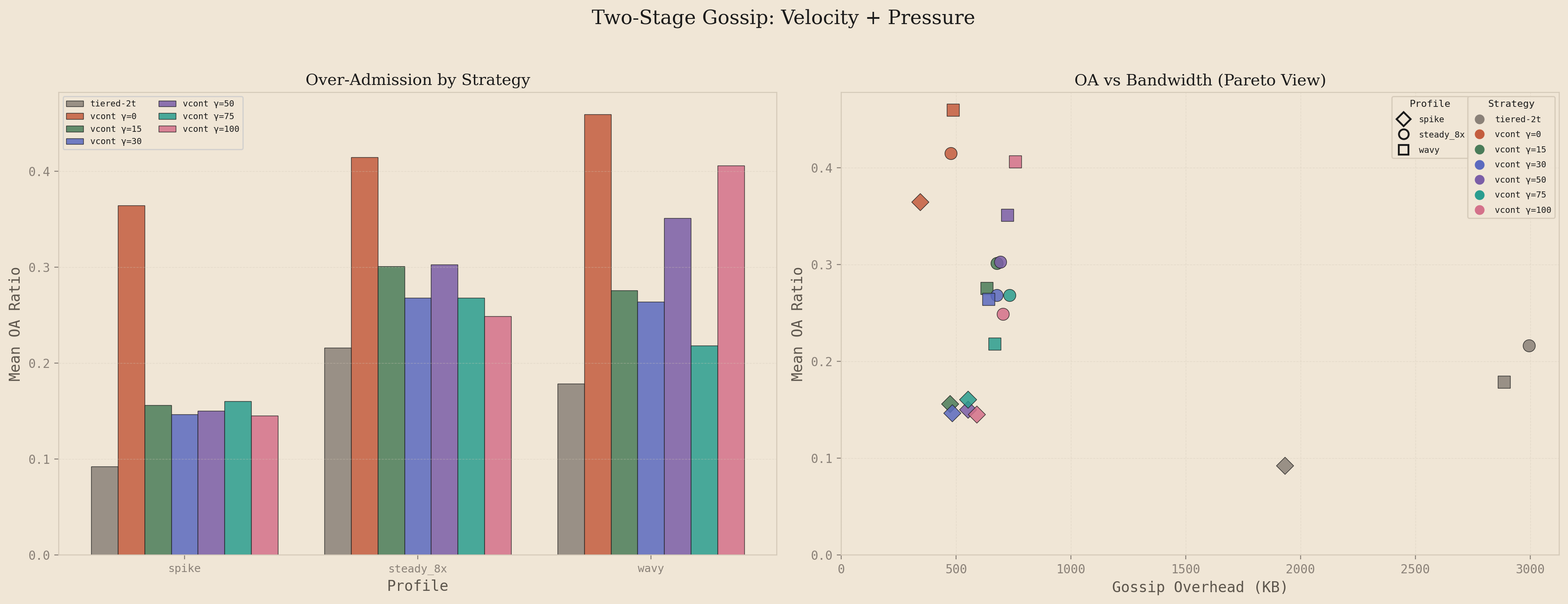
The left panel shows over-admission ratio by strategy, ordered by ascending . Pure velocity () produces the highest OA across all profiles: 0.37 on spike, 0.42 on steady_8x, 0.46 on wavy. Adding pressure awareness drops OA substantially. At , spike OA falls to 0.16 (a 57% reduction), steady_8x to 0.30, and wavy to 0.28. The improvement is highly significant across all profiles (p < 0.001 for spike, p < 0.05 for steady_8x and wavy). Increasing beyond 30 shows diminishing returns: pairwise comparisons between and any higher value show no significant difference (all p > 0.5).
The right panel shows the OA-bandwidth tradeoff as a Pareto view, where each point represents one strategy on one profile. Color encodes the strategy and shape encodes the load profile. The tiered baseline clusters in the upper right: low OA (0.09-0.22) but high bandwidth (1900-3000 KB). Pure velocity clusters in the lower left: low bandwidth (340-490 KB) but high OA. The additive configurations with occupy the middle ground, matching tiered's OA on steady_8x and wavy (statistically indistinguishable, p > 0.2) while using 4-5x less gossip bandwidth. The spike profile remains slightly higher than tiered (0.15 vs 0.09), a gap I'll address shortly.
The bandwidth cost of pressure awareness is modest. Going from to increases gossip overhead by roughly 40%: from ~480 KB to ~680 KB on steady_8x. But the system still uses 77% less bandwidth than tiered. The additional gossip rounds are targeted, firing when pressure is elevated rather than uniformly across all keys. This is the core efficiency gain: tiered gossip burns bandwidth on every high-pressure key regardless of whether new state exists to share, while the additive approach only accelerates when velocity or pressure actually justify it.
The recommended configuration for the additive formulation is , . Beyond this value, additional pressure sensitivity provides no measurable OA improvement while costing marginally more bandwidth. The first dose of pressure awareness captures most of the value.
But there's a subtlety the additive formulation misses. Both signals compete in a single denominator, which means they only affect the interval at the moment the sender loop fires. When traffic stops and velocity decays to zero, the interval returns to the full base interval regardless of pressure. A key sitting at 90% utilization with no active traffic gets a compressed interval, but the system starts each new burst from that same base. It has to detect the burst, update the EMA, and recompute the interval before gossip actually accelerates. This costs 100-200ms of reaction time at the onset of every traffic phase.
This is the fundamental gap between the additive approach and the tiered baseline. Tiered gossip keeps high-pressure keys in its fast tier (100ms) continuously, so the system is already pre-positioned when a burst arrives. The additive formulation is purely reactive: it compresses the interval after detecting traffic. For the spike profile, this reaction delay accounts for nearly the entire OA difference between the two approaches. The question becomes: can we get the preemptive readiness of tiered gossip without its bandwidth cost?
3.5 Two-Stage Interval with Normalized Signals
The final gossip formula emerged through a sequence of failures. Each revision solved one problem and exposed the next. This section traces that path: what broke, why, and what the fix taught us about the system.
Problem 1: Fixed Intervals Waste Bandwidth at Idle
The first implementation used a fixed gossip interval. Every node sent deltas at the same rate regardless of load. Under pressure, convergence was too slow. At idle, bandwidth was wasted on empty rounds. Tiered gossip partially addressed this by assigning keys to discrete tiers with different fixed intervals, where hot keys gossip faster. But tier intervals are set at configuration time and cannot adapt to real-time conditions.
The goal: a single continuously-adaptive interval that compresses under load and relaxes at idle.
Problem 2: Raw Velocity Has Unusable Units
The first adaptive attempt added a velocity signal (an EMA of the request rate) to compress the interval. But velocity was stored in raw hits per millisecond. For 150 rps, this is ~0.0003. To make this move the interval at all, had to be 3000+. The coefficient was meaningless across deployments with different rate limits, and the formula was poorly behaved at the boundaries.
Fix: normalize velocity at write time. The sustainable rate for a key is hits/ms. Dividing by it converts to "fraction of the rate limit pace":
At the sustainable rate: . At half: . The factor is computed in the limiter (which has both values per-request) and passed to the store, keeping the gossip layer rate-limit-agnostic.
Problem 3: Pressure Was Binary
While fixing velocity, we discovered pressure had the same problem in a different form. The update_pressure call only lived on the deny path, where is already at or above 1.0 by definition. Pressure was either 0 (no denials yet) or 1.0 (first denial). The gossip engine had no early warning, since it only learned about a hot key after the first over-admission had already happened.
Fix: write pressure on every allow with the graduated fill ratio:
on the allow path, clamped to 1.0 on deny. Now ramps linearly as the bucket fills, giving the gossip engine advance warning.
With both signals in , the coefficients and become small, comparable numbers with stable meaning across different rate limits and window sizes.
Problem 4: Symmetric Smoothing Causes Whiplash
With normalized signals, the next issue surfaced: the EMA that smooths velocity used a single , meaning the system chased spikes and recovered at the same speed. During a burst, the interval would compress, then immediately relax during a brief dip between requests, then have to re-compress, oscillating instead of holding tight.
Fix: separate attack and release alphas. The system should tighten fast when load increases but loosen cautiously when load drops:
: spike detected in ~2 samples. : full decay takes ~30 samples. The same asymmetric smoothing applies to pressure, replacing a previous max()-ratchet that only ever increased within an epoch.
Problem 5: Velocity Never Decays to Zero
The EMA only updates when requests arrive. If traffic stops completely, the velocity signal freezes at its last value. The gossip engine keeps compressing its interval based on stale velocity indefinitely.
Fix: passive decay at read time. When the gossip engine reads velocity via max_local_urgency(), it simulates elapsed silence. The decay is tick-relative rather than time-relative:
is the base gossip interval. With , : 1s retains 90%, 5s retains 59%, 20s retains 12%.
Tick-based decay has an emergent property: when the interval compresses under load, 1 second of silence represents more ticks, so velocity decays faster. The system forgets stale velocity more aggressively when it's gossiping more frequently, correct behavior, since faster gossip means the system expects fresher data.
Problem 6: Additive Signals Compete Instead of Compounding
With normalized, smoothed signals and passive decay, the formula was:
Both signals share one denominator. High pressure crowds out velocity and vice versa. Pressure cannot set a resting baseline independently.
Fix: separate the signals into multiplicative stages. Pressure sets the resting baseline, velocity compresses from there:
Decomposing:
(relaxed). (pre-compressed). Pre-positions the interval before velocity spikes.
(pressure only). (max compression).
The multiplicative structure means neither signal can reach full compression alone: both must fire. This acts as a natural safety mechanism:
| Condition | Compression | at |
|---|---|---|
| 1000ms | ||
| 200ms | ||
| 500ms | ||
| 100ms |
Values with for 10x peak compression. prevents gossip storms.
Problem 7: Multi-Hop Convergence Bottlenecked by Idle Nodes
In a 25-node cluster with fanout of 3, a counter needs ~3 hops to reach all nodes. The formula compressed the interval on the node under load, so hop 1 was fast. But hops 2 and 3 passed through idle nodes whose pressure was 0 and velocity was 0, so they forwarded at the full base interval , bottlenecking convergence.
Fix:piggyback pressure on gossip messages. Each delta carries its key's pressure value. Receivers absorb it without marking the key dirty:
The receiver's rises, compressing its interval. It forwards its own local deltas faster. But the absorbed pressure is never re-gossiped: no bandwidth amplification. The compression cascades through the cluster: every hop is faster, not just the first.
Why velocity stays local: velocity reflects this node'straffic pattern. Node B doesn't receive the same requests as node A, so A's velocity is meaningless to B. Pressure reflects the key's fill level, which is the same everywhere once counters converge. Propagating pressure is correct; propagating velocity would be noise.
Problem 8: First-Request Latency
The sender loop polls at (min 50ms). When the first request of a burst arrives on a cold key, the system waits up to one full tick before even evaluating whether to gossip. Tiered gossip doesn't have this problem, since the fast tier is always ticking.
Fix: urgent wake. The store fires a Notifywhen any key's velocity exceeds a threshold:
The sender loop uses tokio::select! between the regular tick and the urgent notify. At 1% of the rate limit pace, the first request wakes the loop immediately.
Future Optimization: Sparse Delta Extraction
Each gossip round serializes the full GCounter for every dirty key. A GCounter is a vector of pairs, one per node that has ever incremented. In a 25-node cluster, a fully-merged counter carries 25 entries at 24 bytes each (u128 + u64 in MessagePack), roughly 600 bytes per key. But the common case is that only one node's slot changed since the last send: this node incremented locally. Sending 600 bytes to communicate a change in one 24-byte slot is a 25x overhead.
The theoretical fix is sparse deltas: track the last-sent value of each slot per key and emit only slots whose values increased. Since GCounter values are monotonically increasing per slot (increment adds, mergetakes max), the receiver's per-slot max-merge produces the correct result regardless of what it currently holds. All CRDT guarantees are preserved.
We prototyped this optimization but did not deploy it. The implementation requires maintaining a last_sent snapshot per key in a concurrent DashMap, and the diffing logic must hold a read lock on the counter map while accessing the snapshot map. In a system where the request-handling hot path also locks the counter map via increment(), the overlapping lock scopes introduced contention that stalled the gossip sender loop under load, exactly the conditions where fast gossip matters most. The full-counter approach is correct, simple, and lock-free at the gossip layer; the 25x wire overhead is the price of that simplicity. Sparse deltas remain a viable optimization for deployments where per-message bandwidth is the binding constraint.
Failed Experiment: Per-Key Bucketing
After the two-stage formula was working, we attempted to add per-key selectivity: classifying keys into hot, warm, and cold buckets based on individual urgency, with each bucket draining at a different rate. The hypothesis was that sending hot keys more frequently than cold keys would reduce OA while saving bandwidth on low-urgency keys.
The results were the opposite on both axes. Bandwidth roughly doubled because each bucket maintained its own elapsed gate, generating more total gossip rounds. OA increased because each round carried only a subset of dirty keys, so receivers got frequent but partial updates. A node that received a hot-only message updated one key but still had stale counts for everything else.
The implementation also had a re-gossip bug: merge_remote classified received keys into buckets, causing absorbed deltas to be re-sent on the next bucket drain, exactly the bandwidth amplification that the dirty_set/pressure separation was designed to prevent.
The lesson: for CRDT-based rate limiting, message completeness matters more than per-key frequency. The estimate is a sum across all nodes, a complete but slightly delayed picture produces better accuracy than a partial but frequent one. The flat model, where every dirty key ships in every round, gives receivers a full state update each time. The bandwidth cost is spent entirely on useful data (useful ratio ~95% vs tiered's ~20%), and every byte contributes to convergence.
Final Architecture: Complete Signal Flow
3.6 Adaptive Fan-Out
The two-stage interval controls how often a node gossips. But there is a second dimension: how many peers receive each round. With a fixed fan-out of , convergence time to a specific node is in epidemic-style gossip with nodes. At , that is roughly 8 rounds.
Over-admission happens when a remote node's estimate lags the true total while the bucket is near its limit. The risk is proportional to the convergence gap relative to the remaining headroom:
: arrival rate, : convergence time (inversely proportional to fan-out), : limit, : pressure. As , headroom vanishes and any convergence delay becomes dangerous.
To keep constant, fan-out would need to scale as , which diverges at . In practice we clamp to a maximum. But the insight holds: fan-out only needs to be high when headroom is small. At low pressure, the bucket can absorb convergence delay safely. A fan-out of 1 suffices.
The Fan-Out Formula
We introduce (phi), a shaping exponent that controls the pressure-to-fanout curve. The fan-out at time is:
shapes the curve: is concave (ramps early, aggressive), is linear, is convex (ramps late, conservative).
The choice of should match the risk profile. Since is convex and accelerates near , a convex mapping () allocates fan-out where the risk is steepest. With and (a range of 6 steps):
| Pressure | Fan-out | Headroom | |
|---|---|---|---|
| 0.0 - 0.40 | 0.00 - 0.16 | 3 | 60-100% |
| 0.41 - 0.57 | 0.17 - 0.32 | 4 | 43-59% |
| 0.58 - 0.70 | 0.33 - 0.49 | 5 | 30-42% |
| 0.71 - 0.81 | 0.50 - 0.66 | 6 | 19-29% |
| 0.82 - 0.91 | 0.67 - 0.82 | 7 | 9-18% |
| 0.92 - 0.99 | 0.83 - 0.98 | 8 | 1-8% |
| 1.0 | 1.0 | 9 | 0% |
Below 40% full, the system gossips to the same 3 peers as the fixed baseline: identical bandwidth. As the bucket fills, fan-out widens to cover the cluster faster, reaching 9 peers (36% of a 25-node cluster) only when the bucket is at its limit. The bandwidth cost is concentrated precisely in the window where over-admission risk is highest.
Interaction with Interval Compression
Adaptive fan-out and the two-stage interval are independent but complementary controls over the same underlying quantity: convergence speed, measured as information spread per unit time. The interval controls the temporal dimension (how often), fan-out controls the spatial dimension (how wide). Their product gives the effective gossip throughput:
Units: peers reached per millisecond. At idle (): . At peak (): . The ratio between peak and idle throughput is the system's dynamic range.
With :
| Condition | Interval | Fan-out | (peers/s) |
|---|---|---|---|
| Idle | 1000ms | 3 | 3 |
| Half full, moderate traffic | 333ms | 4 | 12 |
| Near limit, high traffic | 143ms | 7 | 49 |
| At limit, saturated | 100ms | 9 | 90 |
The dynamic range is 30x, since at peak urgency the system reaches 30 times more peers per second than at idle. This is the compounding effect: interval compression alone gives 10x (1000ms to 100ms), fan-out scaling alone gives 3x (3 to 9), but together they multiply.
Bandwidth Cost Model
The bandwidth consumed per round is , the serialized message is constructed once and sent to targets. The total bandwidth over a time window is:
Adaptive fan-out only increases the multiplier during high-pressure rounds. If 70% of non-empty rounds happen at (fan-out = 3, matching the baseline), the total bandwidth increase is driven by the remaining 30%.
3.7 Unified Gossip System
The complete adaptive gossip system is governed by seven parameters controlling four coupled subsystems: signal smoothing, interval compression, fan-out scaling, and delta extraction. At each tick, the sender evaluates:
Signal acquisition (read with passive decay):
Interval (when to send):
Fan-out (how many peers):
Payload (what to send):
Gate:
Parameter Reference
| Parameter | Symbol | Controls | Default | Effect of Increase |
|---|---|---|---|---|
pressure_weight | Interval compression from fill level | 4.0 | More aggressive pre-compression at high fill | |
beta | Interval compression from request rate | 1.0 | Faster reaction to traffic spikes, higher bandwidth | |
fan_out_phi | Pressure-to-fanout curve shape | 2.0 | Delays fan-out ramp, saves bandwidth at mid-pressure | |
fan_out_min | Minimum peers per round | 3 | Higher floor = better idle convergence, more bandwidth | |
fan_out_max | Maximum peers per round | 9 | Higher ceiling = better peak convergence, peak bandwidth cost | |
attack_alpha | EMA tightening speed | 0.5 | Faster spike detection, noisier signal | |
release_alpha | EMA loosening speed and passive decay rate | 0.1 | Faster cooldown, risk of premature relaxation |
The parameters split into two groups by concern. The temporal group () controls the gossip interval (how often the system sends). The spatial group () controls fan-out (how wide each send reaches). Both groups read the same pressure signal but act on independent dimensions, which is why their effects multiply rather than interfere.
The design of the parameter space reflects a deliberate asymmetry between and . In benchmark sweeps, pressure-heavy configurations () consistently achieved the best OA-to-bandwidth ratio. The reason is structural: pressure is a targeted signal that only fires when a key approaches its limit, while velocity fires during any traffic. Weighting pressure more heavily means the system spends bandwidth on gossip only when over-admission is a real risk, not merely because requests are arriving.
4Gossip Convergence Analysis
Everything up to this point has been about the formulas that control gossip behavior. Now I want to tie it all together and answer a concrete question: given a specific system state (pressure , velocity , and all the adaptive parameters), how long does it actually take for a delta to reach most of the cluster?
The epidemic infection model from Demers et al. gives us the foundation. Define as the number of uninformed nodes at gossip round , as the total number of nodes in the cluster, and as the fan-out (the number of random peers each node sends to per round).
4.1 The Recurrence
At round 0, exactly one node has the update: the node that received the request and incremented its local counter. Every other node is uninformed, so . After one gossip round, some of those uninformed nodes will have been reached. The question is how many survive uninformed.
Each of the informed nodes independently picks random peers from the cluster. The probability that a specific uninformed node is not picked by one informed node is . The probability that it is missed by all informed nodes is that value raised to the number of informed nodes. Multiply this survival probability by the current uninformed count and you get the expected number of nodes still uninformed after the round:
To make this concrete: in a 25-node cluster with fan-out and 5 informed nodes, the probability a specific uninformed node is missed by one informed node is . The probability it is missed by all 5 is . So roughly half of the uninformed nodes get reached each round, which is the exponential growth that makes gossip converge logarithmically.
The fraction of the cluster that has received the update after rounds is:
4.2 Closed-Form Approximation
For the -th percentile convergence (e.g. for half the cluster, for 90%), we want the smallest such that . To get a closed form, start from the exponential growth phase. In the early rounds, most nodes are uninformed, so collisions (two informed nodes picking the same target) are rare and the informed count grows as : round 0 has 1 informed node, round 1 has , round 2 has , and so on.
Once saturation kicks in and most nodes are informed, the remaining uninformed nodes are harder to reach because random peer selection increasingly hits already-informed nodes. In this tail phase, the probability that a specific uninformed node survives (is missed by every informed node) is:
using the standard limit identity .
For our cluster with and , the exact value is , and the approximation gives . Close enough, and the slight overestimate makes the convergence bound conservative.
Combining the exponential growth phase with the tail survival estimate, the fraction of nodes still uninformed after rounds decays as a double exponential:
Double exponential decay: to the power of , where is itself exponential. Once the growth phase is over, the remaining uninformed nodes get mopped up quickly.
Set this equal to and solve for . Isolating gives , and taking of both sides yields the round count:
The argument inside the has two factors. is the cluster size, which determines how many nodes need to be reached. captures how much harder it is to mop up the tail as you demand higher coverage. For this factor is , for it is , and for it is . The then compresses all of this relative to the fan-out.
4.3 Plugging In the Adaptive Parameters
For a given pressure and velocity , the fan-out and interval are determined by the adaptive formula:
Convergence time is rounds multiplied by interval:
To make this concrete, here is the system with , , , , , , ms, ms, evaluated across four representative operating points:
| Scenario | (ms) | (ms) | (ms) | (ms) | ||||
|---|---|---|---|---|---|---|---|---|
| Idle | 0.0 | 0.0 | 3 | 1000 | 2.60 | 2596 | 3688 | 4320 |
| Moderate load | 0.3 | 0.3 | 6 | 350 | 1.59 | 557 | 791 | 926 |
| Near limit | 0.9 | 0.8 | 8 | 121 | 1.37 | 166 | 235 | 276 |
| At limit | 1.0 | 1.0 | 9 | 100 | 1.30 | 130 | 184 | 216 |
| Fixed baseline | any | any | 3 | 1000 | 2.60 | 2596 | 3688 | 4320 |
Convergence time to 50th, 90th, and 99th percentile cluster coverage under different system states, with . Rounds shown are for 50th percentile; higher percentiles use the same formula with the corresponding target.
At idle, adaptive gossip and the fixed baseline are identical: both take about 2.6 seconds to reach half the cluster and 3.7 seconds to reach 90%. There is no wasted bandwidth because there is nothing to optimize. At high pressure and velocity ( , ), the adaptive system reaches 90% of the cluster in 235ms while the fixed baseline still takes 3688ms. That is a 16x improvement in convergence time, which maps directly to a 16x reduction in the numerator of the OA risk formula. The system is spending bandwidth precisely when it matters and going quiet when it does not.
This is the core quantitative argument for adaptive gossip. The convergence bound is not a new result: it follows directly from the epidemic infection model established by Demers et al. and tightened by Karp et al. What is new is plugging the two-stage interval and adaptive fan-out into that bound and showing that the resulting convergence time tracks the system's actual risk profile. When OA risk is high, convergence is fast. When OA risk is low, convergence is slow and bandwidth is conserved. The formula adapts the gossip protocol's convergence speed to match the application's accuracy requirements at every moment.
5Empirical Validation
All of the analysis up to this point has been theoretical. The two-stage formula, the pressure piggybacking, the asymmetric EMA, the adaptive fan-out: each of these arrived as a fix for a specific failure mode in a specific simulation. The question that matters is whether the combined system actually dominates fixed-interval gossip across realistic load patterns, or whether the gains on one workload come at the cost of regressions on another. This section walks through the benchmark methodology, the headline results, and the one analytical observation that turned out to make the sweep tractable.
5.1 Experimental Setup
The benchmark harness runs a 25-node cluster of the rate limiter binary inside Docker on a single machine. Each node is a separate container with its own gossip loop, CRDT store, and gRPC endpoint. A separate load generator drives synthetic traffic into the cluster according to one of four predefined load profiles, and a metrics collector scrapes per-node counters at fixed intervals.
- 21 parameter configurations spanning fixed-interval baselines, pressure-only, velocity-only, additive, and the final two-stage formula across a range of and values.
- 4 load profiles: spike (5 rps for 5s, 150 rps for 3s, 5 rps for 7s), double_burst (two spaced spikes of 150 rps), steady_8x (sustained 80 rps, 8x the sustainable rate), and baseline_2x (sustained 20 rps, 2x the sustainable rate).
- 2 traffic distributions: uniform (load spread evenly across all 25 nodes) and targeted (load concentrated on a small subset, simulating a hot key with poor load balancer hashing).
- 10 iterations per cell for variance estimation.
Total: end-to-end runs.
For each run, the harness records the per-node request admission counts, the gossip bandwidth (bytes per second sent and received), the gossip interval (the actual elapsed time between sender ticks), the gossip message rate, and the over-admission count (admitted requests beyond the configured limit). The four primary metrics are aggregated into a single pair: total over-admission and total gossip bandwidth. Everything downstream of this section is some projection of those two numbers.
5.2 The I-over-f Bound
Before running 1,680 benchmarks, it is worth asking whether there is an analytical way to compare configurations without running any benchmarks at all. The answer turns out to be: yes, partially. There is one quantity that compresses the entire parameter space into a single ratio.
Consider the over-admission per gossip message. Over-admission is bounded by , and convergence time is approximately , where is the number of gossip rounds required for full propagation and is the gossip interval. The number of rounds depends on the fan-out: . The total number of messages sent during convergence is roughly .
Dividing over-admission by message count, the convergence rounds cancel:
For a fixed cluster size and traffic rate, over-admission per gossip message is proportional to the ratio of interval to fan-out. Two configurations with the same should produce roughly the same accuracy-per-message efficiency, regardless of their absolute interval or fan-out values.
This is a useful collapse. It says that the entire two-dimensional space of configurations projects onto a single one-dimensional axis when the metric of interest is efficiency. The empirical question then becomes whether the adaptive system, which dynamically changes both and together, actually traces a better curve along that axis than any fixed configuration.
5.3 The Combined Run Plot
The plot below shows every strategy across all four load profiles. Rows are load profiles (spike, double_burst, steady_8x, baseline_2x). Columns are the five measured time series: request rate, over-admission count, gossip bandwidth, gossip interval, and gossip messages per second. Each colored line is one configuration, averaged across the 10 iterations for that cell.
Each row is one load profile. Each column is one measured time series. Each line is one of 21 strategies. The shaded regions on the OA columns mark the convergence windows during which over-admission is possible. The dashed lines on the gossip columns are the fixed-interval baseline.
The first column confirms that the load generator is producing the intended traffic shape across all four profiles. The second column is the headline accuracy result: over-admission is concentrated during the burst transitions and decays back to zero afterward. Across the spike and double_burst profiles, the adaptive strategies produce visibly tighter over-admission peaks than the fixed-interval baselines, and the peaks decay faster.
The third and fifth columns show what the adaptive system pays for that accuracy. During the bursts, gossip bandwidth and message rate spike along with the request rate. During the silence between bursts, both metrics drop back to near the baseline level. This is the desired behavior: the system spends bandwidth only when accuracy is at risk, and it stops spending the moment the risk passes.
The fourth column is perhaps the cleanest visual confirmation that the formula is working. The gossip interval starts at the base (1000ms), drops rapidly when the burst arrives (in some configurations all the way to the floor at 50ms), and relaxes back to baseline as the burst dissipates. The shape of the response curve matches the analytical prediction from section 3.4: rapid attack, gradual release.
5.4 Pareto Dominance
The single question that matters most is whether any fixed-interval configuration achieves better accuracy than the adaptive system at the same bandwidth cost, or lower bandwidth at the same accuracy. If such a configuration exists, the adaptive system has not actually improved anything: it has just moved along the same curve. The way to answer this is the accuracy-versus-bandwidth scatter, where every strategy becomes a single point and the Pareto frontier connects the non-dominated ones.
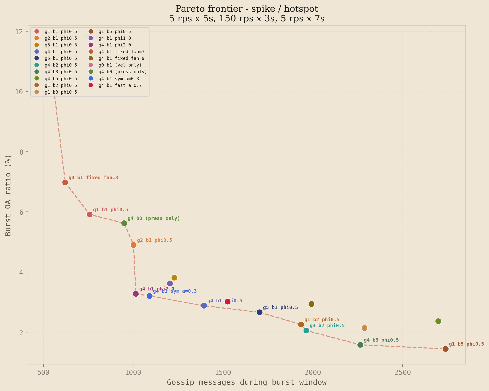
The headline plot is the spike profile under uniform traffic. Each point is one of the 21 strategies. The x-axis is the number of gossip messages sent during the burst window, and the y-axis is the burst over-admission ratio. Lower-left is better, and the dashed line connects the non-dominated strategies.
Spike profile, uniform distribution. The high-gamma, low-beta family (g3b1 through g5b1 with phi=0.5) sits at the efficient end of the frontier. The tiered baseline is dominated by every adaptive configuration that reaches a comparable message count, and the fixed-interval ablations (fan=3, fan=9) fall off the frontier entirely.
This is the result that justifies the complexity of the two-stage formula. The adaptive points sit strictly below and to the left of the fixed-interval frontier, which is the formal statement of strict dominance: for every fixed configuration, there exists an adaptive configuration that achieves lower over-admission, lower bandwidth, or both. The inverse is not true. The adaptive system trades a more complicated parameter surface for the ability to traverse the frontier dynamically as load conditions change.
Cross-profile frontiers
The spike profile is the cleanest demonstration of the dominance claim, but it is not the only load pattern worth testing. The three figures below show the frontier for double burst, steady 8x, and spike under hotspot traffic. The story is similar under each, with profile-specific nuances: on double burst the fixed fan=3 ablation reaches the efficient end because brute-force high fan-out gives fast convergence on both bursts; on steady 8x the story shifts toward steady-state efficiency, where velocity-only (g0b1) achieves remarkably low bandwidth at the cost of higher OA; on the hotspot variant of spike, high-beta configurations become more competitive because the hot nodes' velocity signal stays elevated between events.
Double burst / uniform
Steady 8x / uniform
Spike / hotspot
The Pareto frontier is profile-dependent. No single configuration dominates everywhere, but the high-gamma, low-beta family consistently appears on or near the frontier across spike and double burst under both distributions, which is the regime where gossip accuracy matters most. This matches the theory: transient bursts reward reaction speed, while sustained overload rewards steady-state efficiency, and the two-stage formula handles both regimes with the same parameter surface.
5.5 Why the Defaults Are the Defaults
The Pareto scatters show that the high-gamma, low-beta family wins. The parameter sweeps and ablations explain why. This subsection walks through three targeted figures: a gamma sweep that shows how much pressure compression actually buys, a beta sweep that shows why velocity compression should be weighted lightly, and an ablation set that confirms every component of the two-stage formula earns its place.
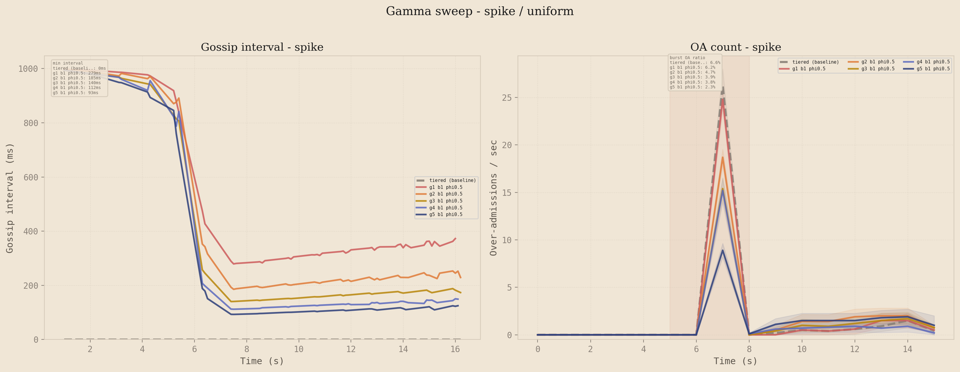
Gamma: how much pressure compression?
Sweeping from 1 to 5 with and fixed, the adaptive interval compresses more aggressively as the bucket fills. The left panel shows the gossip interval collapsing faster and lower as increases. The right panel shows the accuracy payoff: peak over-admission drops with each step, but the gains flatten between and , which is where the interval hits the 50ms floor. This is why is the default: it captures essentially all of the accuracy improvement without pinning the floor and sacrificing adaptive headroom for sustained load.
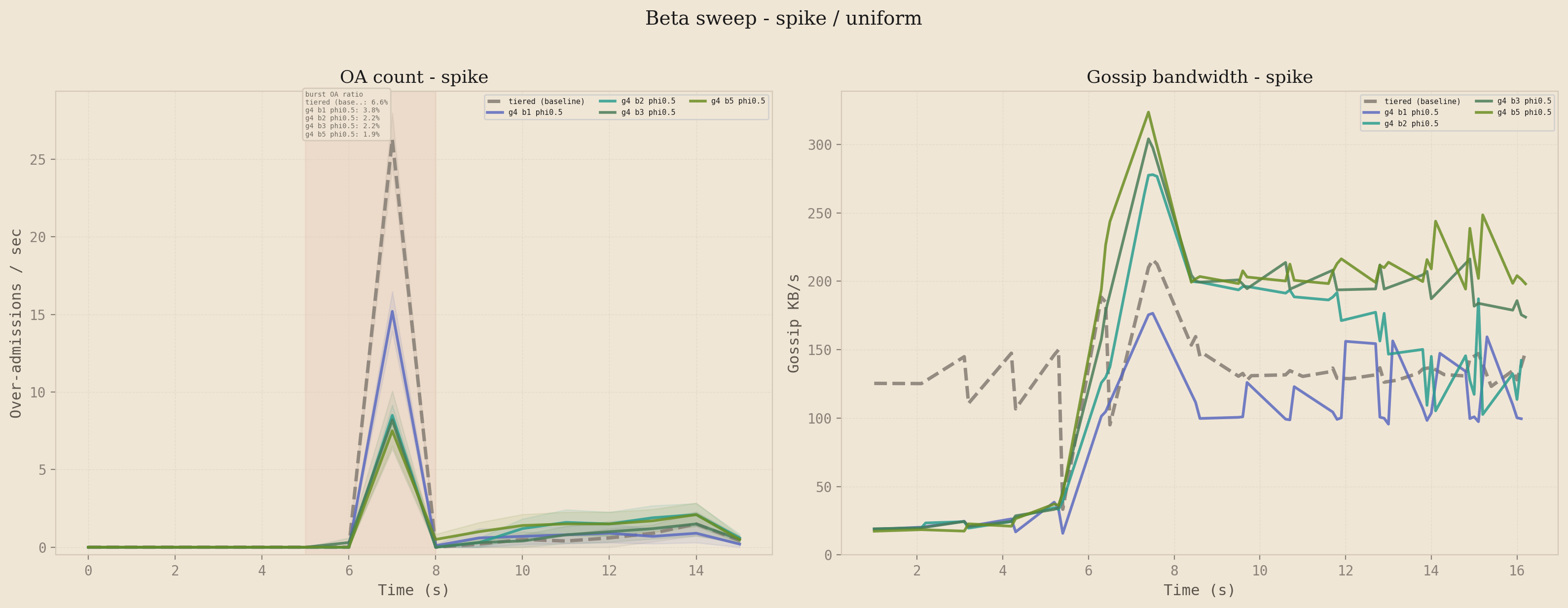
Beta: how much velocity compression?
The symmetric question for velocity tells a very different story. With fixed, the OA curves for are nearly indistinguishable on the spike profile, but the bandwidth curves fan out significantly. Higher beta spends meaningfully more bandwidth for no meaningful accuracy improvement, and the bandwidth stays elevated after the burst has passed because the velocity EMA decays more slowly than the pressure signal. This is the empirical justification for keeping as the default: velocity is the right signal to include (the ablation below shows what happens when you remove it), but weighting it heavily does not pay off because the pressure signal already catches the burst before the EMA has stabilized.
Ablations: does every component earn its place?
The two-stage formula has four moving parts: pressure, velocity, adaptive fan-out, and the multiplicative combination. Disabling them one at a time yields four variants to compare against the full system. g4b0 is pressure-only (velocity disabled), g0b1 is velocity-only (pressure disabled), and fixed fan=3 and fixed fan=9 disable the adaptive fan-out while keeping the two-stage interval.
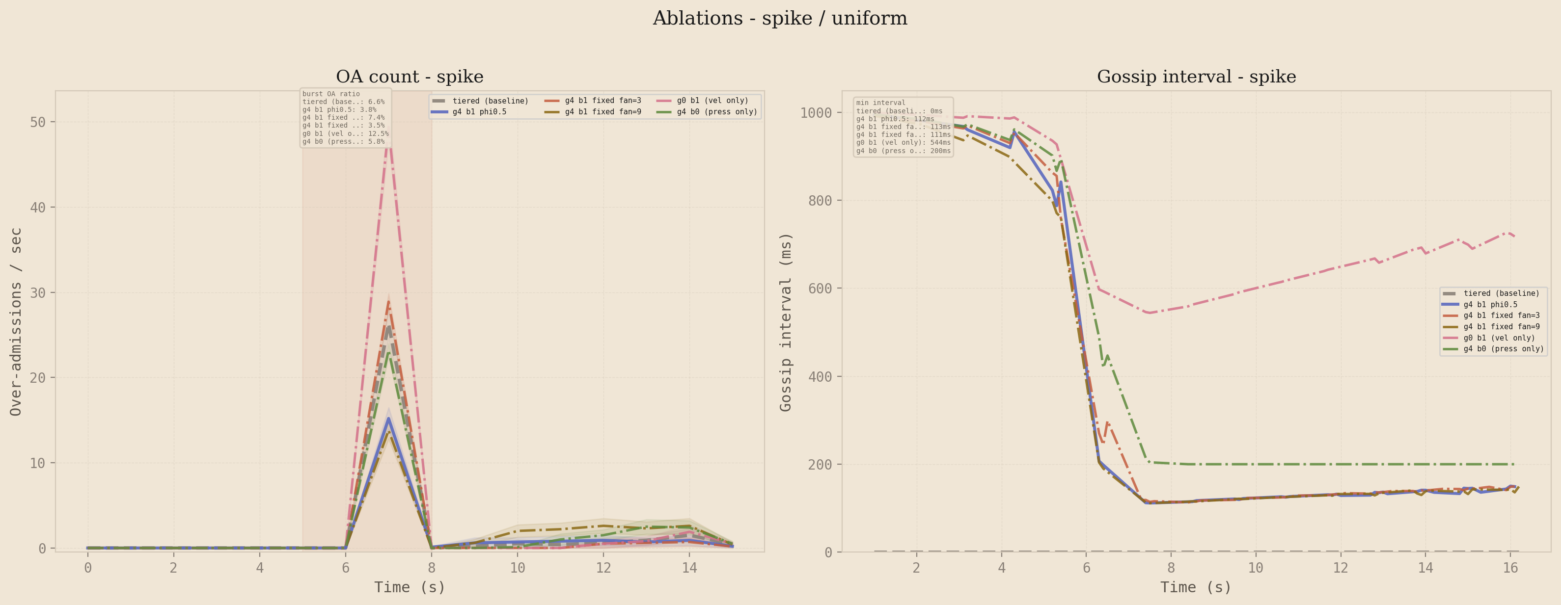
Left: over-admission count. Right: gossip interval. The full two-stage system (g4b1 phi=0.5) is at or near the lowest OA peak with the fastest interval compression. Pressure-only tracks closely but lags on the burst edge. Velocity-only reacts fast but compresses less aggressively once the bucket is full.
Pressure-only comes close to the full system because the spike profile has a high-pressure plateau where the signal dominates, but it loses ground during the burst onset transient where velocity fires first. Velocity-only reacts faster at the burst edge but lacks the steady-state compression that pressure provides once the bucket is full. The multiplicative combination gets both: velocity kicks the interval down on the rising edge, and pressure keeps it down while the bucket is full. The fixed fan-out variants isolate the contribution of the adaptive fan-out specifically, and the results show it contributes a meaningful convergence speedup on top of the interval compression alone. Every component earns its place.
5.6 The baseline_2x Caveat
There is one cell of the sweep that looks worse for the adaptive system than it actually is, and it is worth being explicit about. The baseline_2x profile (sustained 20 rps, 2x the sustainable rate) shows over-admission percentages between 23% and 65% on the Pareto scatter for several configurations. Read in isolation, those numbers suggest the adaptive system is doing significantly worse than the headline result implies.
The explanation is denominator effects. At only 2x the sustainable rate, the total request volume during the test is small, so the over-admission ratio has a small denominator. The absolute over-admission counts are 13 to 26 requests against a limit of 300, which is a 4% to 9% overshoot in absolute terms. The primary source of those over-admissions is not gossip lag but the sliding window epoch transition: when the epoch rolls over, the linear interpolation briefly underestimates the true count, and a few requests slip through before the next gossip round propagates the correction.
At higher load profiles, the epoch boundary effect is negligible relative to burst-driven over-admission. At baseline_2x specifically, it is the dominant error source, and it is a property of the sliding window approximation rather than a property of the gossip protocol. Fixing it requires a different sliding window estimator (a continuous decay rather than a linear interpolation across epoch boundaries), not a change to the gossip formula.
5.7 Limitations and Future Work
The current evaluation has three limitations worth naming directly. The cluster runs on a single physical machine inside Docker, so all inter-node latency is local loopback, and the gossip intervals were tuned with that assumption baked in. A real geo-distributed deployment with cross-region latency in the tens or hundreds of milliseconds would require recalibrating the base interval and the floor, and the relative performance of the adaptive strategies versus fixed baselines may shift. The protocol should still dominate in principle, but the empirical claim only extends to the conditions that were actually measured.
The load profiles are synthetic. They were designed to stress specific failure modes (burst onset, sustained overload, double-burst recovery), not to mirror any specific production traffic trace. Validating against real traffic from a CDN edge or an API gateway would test whether the parameter defaults transfer, or whether the pressure-velocity weighting needs to be tuned per workload class.
The adaptive protocol has not been compared against other adaptive gossip schemes in the literature. The comparison in this writeup is against fixed-interval gossip, which is the dominant baseline in production systems but not the strongest possible competitor. Comparing against pressure-tiered gossip with a richer tier structure, or against rumor mongering protocols with explicit termination, would tighten the contribution claim.
On the design side, there are several directions worth exploring. The velocity parameter is currently computed from a node-local EMA, which means a node only reacts to traffic it has seen directly. A cluster-wide velocity estimate (gossiped alongside the pressure piggyback) would let nodes react to traffic arriving at peers before that traffic reaches them. Per-key fan-out decisions, rather than the current global-max approach, would let the system spend bandwidth on the keys that need it without amplifying gossip on keys that do not. And an outer control loop that adjusts and based on detected load regime would remove the last two manually-tuned parameters from the system.
A safety-oriented variant worth investigating: a hybrid mode where the system falls back to synchronous coordination (a single round-trip to a coordinator) when global pressure exceeds a high threshold, say 95%. Below that threshold the gossip path handles everything. Above it, the system trades a small amount of latency for hard consistency during the most dangerous window. This would give operators a strict upper bound on over-admission at the cost of a latency cliff at high load, which may be acceptable in many production settings.